library(tidyverse)
library(openxlsx)
library(kableExtra)
library(scales)
library(numform)
library(flextable)

options(scipen = 999)

Handout 09
Date: 2022-11-27
Topic: Hypothesis Testing

Literature
Handout
Ismay & Kim (2022) Chapter

Testing of hypotheses: the concepts

Introduction: example of formulating a research hypothesis

As part of a research on the economic effects of the outcome of the Brexit referendum in June 2016 the effect on house values in London is investigated. Because of the outcome of the Brexit referendum, the values of houses in London are expected to decrease. This is especially the case in the central districts of London, e.g. the City of Westminster district.
A sub research question is: what is the effect of the Brexit referendum on house values in the City of Westminster district in London.
To investigate the effect of the Brexit referendum on the values of houses in the City of the Westminster district, a comparison is made between the values in January 2016 and the values in January 2017, i.e. a half year before and a half year after the referendum.
As a measurement for the value of the houses, the selling prices of houses sold are used as an indicator. This means that the houses sold are considered to be a random sample of all houses in this district. Due to the outcome of the referendum, a decrease of the house values is expected.
There are many ways to operationalize this assumption. E.g. compare the average selling price in January 2016 with the average selling price in January 2017. Another possibility, and maybe a better choice, is to use the medians. It’s also possible to operationalize the assumption by comparing the proportion of houses sold for which the selling price is above 1 mln GBP. If house prices are decreasing it might be expected that the proportion of houses for which the selling price is more than 1 mln GPB, is decreasing as well. The price paid data for houses sold are collected from the open data at www.gov.uk. In the boxplots in Figure 1 the prices in January 2016 and January 2017 are compared. The median of the house prices in January 2017 is lower than in January 2016, the spread in the prices in January 2017 seems to be lower than in January 2016.
Table 2 gives an overview of some sample statistics. Indeed the average selling price in January 2017 is less than in January 2016.

Figure 9.1 Boxplots selling prices houses (GBP) in City of Westminster district in London

hp_cow <- read.csv("Datafiles/HP_London_jan161718.csv") %>% 
  filter((year == 2016 | year == 2017), district == "CITY OF WESTMINSTER",
         property_type != "O")

hp_cow_summary <- hp_cow %>%
  group_by(year) %>% 
  summarize(COUNT = n(),
            AVERAGE = round(mean(price_paid), -2),
            MEDIAN = round(median(price_paid), -2),
            SD = round(sd(price_paid),-2),
            NUMBER_ABOVE_1MLN = sum(price_paid >= 1E+06),
            PERC_ABOVE_1MLN = round(100*NUMBER_ABOVE_1MLN/COUNT,1))

hp_cow %>% 
  ggplot(aes(y= factor(year), x = price_paid)) +
  geom_boxplot(fill = "royalblue") +
  xlab("Price Paid in GBP") +
  ylab(NULL) +
  scale_x_continuous(labels = comma) +
  theme_minimal()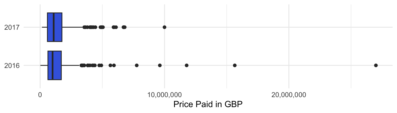

Note. A comparison is made between the selling prices in January 2016 and in January 2017.

Table 9.1
Summary statistics prices houses sold in London, City of Westminster district in January 20016 and January 2017

M2016 <- format(hp_cow_summary[[1,3]], big.mark = ",")
SD2016 <- format(hp_cow_summary[[1,4]], big.mark = ",")
M2017 <- format(hp_cow_summary[[2,3]], big.mark = ",")
SD2017  <- format(hp_cow_summary[[2,4]], big.mark = ",")
ttest <- t.test(hp_cow$price_paid[hp_cow$year == 2017 & hp_cow$property_type != "O"],
                hp_cow$price_paid[hp_cow$year == 2016 & hp_cow$property_type != "O"],
                alternative = "less")
tvalue <- round(ttest$statistic, 3)
pvalue <- round(ttest$p.value, 3)

names(hp_cow_summary) <- toupper(names(hp_cow_summary))

flextable::flextable(hp_cow_summary) %>% 
  width(j = 1:2, width = .5) %>% 
  width(j = 3:7, width = 1) %>% 
  colformat_num(j = c(1, 2, 4), digits = 0) %>% 
  colformat_num(j = c(3, 5), big.mark = ",", digits = 0)

YEAR	COUNT	AVERAGE	MEDIAN	SD	NUMBER_ABOVE_1MLN	PERC_ABOVE_1MLN
2,016	333	1,490,100	999,000	2,042,500	164	49.2
2,017	236	1,478,800	1,087,500	1,394,700	123	52.1

Note. Average, median and standard deviation (SD) are in GB Pounds. The last column gives the percentages of properties sold with a selling price above 1 mln GPB. Underlying data are retrieved from http://landregistry.data.gov.uk/app/ppd/.

If the proportion houses for which the selling price is above 1 mln GPB is used as metric for the house values, no support is found for a decrease in these values. After all the proportion with a selling price above 1 mln GPB increased.
The average selling price decreased. It is not unexpected that the two averages differ, because two more or less random groups are compared. Actually it would be very surprising if the two averages would be exactly the same. A lower mean selling price in January 2017, doesn’t necessarily mean that the average value of all houses in the district in January 2017 is lower than the average value in January 2016. The question is whether this difference between the two means is merely a matter of chance, or whether it is due to an underlying difference between the values in January 2017 and in January 2016. To find out if the difference is just a matter of chance, a so-called t-test can be used. The conclusion would be that the outcome of a t-test does not support the assumption that the mean value of houses in the city of Westminster district in January 2017 (M = 1,478,800; SD = 1,087,500) is less than in January 2016 (M = 1,490,100; SD = 999,000); t(566 ) = -.079; p = 0.469.

Hypotheses testing the concepts

Hypotheses testing in court

In a trial there is a statement (hypothesis) the prosecutor wants to prove: ‘the defendant is guilty’. As long as there is no evidence, the opposite is accepted: ‘the defendant is not guilty’. The defendant is found guilty only if the evidence that he is, is ‘beyond reasonable doubt’. After the trial there are four possibilities:
1. The defendant is not guilty and is found not guilty (right decision)
2. The defendant is not guilty, but is found guilty (wrong decision)
3. The defendant is guilty but is not found guilty (wrong decision)
(note: ‘not found guilty’ is not the same as found ‘not guilty’)
4. The defendant is guilty and is found guilty (right decision)

		WHAT IS REALLY TRUTH
		not guilty	guilty
DECISION	Acquitted	right decision	wrong decision, second order error
DECISION	Sentenced	wrong decision, first order error	right decision

Hypotheses testing in statistics

The principles for statistical testing of hypotheses are the same as these in court. The difference is that we are looking for statistical evidence instead of juridical. The researcher postulates a hypothesis he wants to prove, the so called H_A (or H₁) hypothesis. As long as there is no statistical evidence that this hypothesis is true, the opposite (the H₀ hypothesis) is assumed to be true. After a testing procedure the researcher comes to the decision whether to reject or not reject the H₀-hypothesis. In the same way as in court there are four possibilities, shown in the diagram below.

		WHAT IS REALLY TRUTH
		H₀ is right	H₀ is not right
DECISION	Do not reject H₀	right decision	wrong decision, second order error (\(\beta\)-risk)
DECISION	Reject H₀	wrong decision, first order error (\(\alpha\)-risk)	right decision

In a statistical procedure, we examine whether there is statistical evidence that the data contradict the H₀-hypothesis in favor of the H_A. If that is the case the H₀-hypothesis is rejected. Statistical evidence means that the \(\alpha\)-risk may not be greater than a pre-agreed value (usually 0.05). If the statistical evidence is not strong enough to reject the H₀, we stay at the starting point of the procedure (H₀ is true) and we do not reject H₀. This does not mean that there is statistical evidence that supports H₀, it does mean that there is no statistical reason to reject H₀.
The way these statistical procedures are used in various statistical tests is discussed in what follows.

Proportion tests or binomial tests

As can be seen in the above example (house values in London) it is sometimes possible to operationalize a research question by using proportions and formulate a hypothesis about these proportions.

Binomial Experiments

Experiments with two possible outcomes - often denoted as “Success” and “Failure”” - are called Bernoulli experiments.
Repeating a Bernoulli experiment n times with the same probability p of success for each attempt is called a binomial experiment.

Binomial test against a standard

In a univariate analysis a test against a standard is in many cases a good technique to operationalize a research question. Some examples.

Example: predicting the outcome of flipping a coin (1)
Consider a person who claims to be clairvoyant (paranormal gifted) so that he can predict the outcome of flipping a coin.¹

Experiment: ask the person to predict the outcome if the coin is flipped once.
Questions:
(i) If the predition is correct, would that be seen as support for the claim?
(ii) What if the experiment is flipping the coin twice and both predictions are correct?
(iii) What if the coin is flipped three times and all predictions are correct?
(iv) After how many correct predictions can the claim be honored?

Example: predicting the outcome of flipping a coin (2)
Consider a person who claims to be clairvoyant, and says he can better predict the outcome of flipping a coin than simply by guessing. In other words, the claim is that his predictions are correct in more than 50% of the cases.
Research experiment (data collection): the person is asked to make 100 predictions. Based on the number of correct predictions (k) it will be decided to honour his claim or not.
The hypothesis to test is H_A: p > .5 where p is the probability of a correct prediction. In the procedure we start with the assumption that the claim is not correct, in other words p = .5. This is called the H₀-hypothesis.
The set of possible outcomes of the experiment are divided in two groups. One group for which the H₀-hypothesis is not rejected and one group for which the H₀-hypothesis is rejected in favour of the H_A-hypothesis. The last group is called the Critical Region, because an outcome in this group can lead to a first order error.
The partition in two groups is made so that the probability that a first order error is made is at most a pre-determined value \(\alpha\), the significance level of the test. The most common value used is \(\alpha\) = .05.

To come to a decision, that is to determine whether a test result lies in the critical region or not, the so called prob-value will be calculated, that is the probability to find a result as has been found, or even further away from what is expected, assuming p = .5 (i.e. assuming H₀ is true).
If this prob-value is low, than there are two options:
- the probability of a correct prediction is .5, the person was just lucky in guessing correct a great number of times;
- the probability of a correct prediction is more than .5, and that is why the predicted correct a great number of times.
If the prob-value is lower than the pre-agreed \(\alpha\) value the first option is rejected and it is said that the data support the H_A-hypothesis.

For instance if he predicts correctly 60 out of 100 times the prob-value equals 0.028. The prob-value has been calculated using the R function pbinom(). Another way to calculate this prob_value is by writing code to simulate the experiment assuming H₀ is true, repeat this simulations many times (e.g. 10,000) and calculate the proportion of times that 60 or more simulated guesses out of 100 are correct. See the R script

Figure 9.2
Binomial distribution with n = 100, p = .50

n <- 100
k <- 0:100
p <- 0.5
probs <- dbinom(x = k, size = n, prob = p)
df <- data.frame(k, probs)
ggplot(df, aes(k, probs)) +
  geom_bar(data = df[20:60, ], stat = "identity", fill = "lightgrey") +
  geom_bar(data = df[61:80, ], stat = "identity", fill = "black") +
  theme_minimal() +
  xlab("number of correct predictions") +
  ylab("probability") +
  scale_x_continuous(breaks = seq(0,80,2))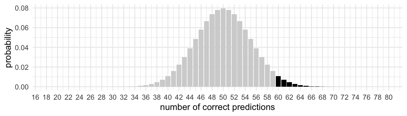

Note. The black area corresponds with the probability of 60 or more successes in 100 trials under the assumption that a probability of a success equals 0.50.

Example: filling packages of sugar
Packs of sugar are filled using a filling machine. Although on average the contents is 1000 gram there is always some variation in the contents of the packs of sugar. In the past 10% of the packages contain less than 995 grams. This was reason to buy a new packing machine. To test if this machine performs better than the old one, a random sample of 100 packs is drawn. From these packs, 6 contain less than 995 grams. Does this sample result give statistical evidence that the machine performs better? In other words: is this sample result enough evidence that in the population less than 10% of the packages contain less than 995 grams.

To answer this question we assume the null-hypothesis - H₀: 10% of the packages contain less than 995 grams - to be true and calculate the probability to find 6 or less packs with less than 995 grams under this assumption.

Figure 3
Binomial distribution with n = 100, p = .10

n <- 100
k <- 0:100
p <- 0.1
probs <- dbinom(x = k, size = n, prob = p)
df <- data.frame(k, probs)
ggplot(df, aes(k, probs)) +
  geom_bar(data = df[1:7, ], stat = "identity", fill = "black") +
  geom_bar(data = df[8:30, ], stat = "identity", fill = "lightgrey") +
  theme_minimal() +
  xlab("number of packs containing less than 995 gram") +
  ylab("probability") +
  scale_x_continuous(breaks = seq(0,30,2))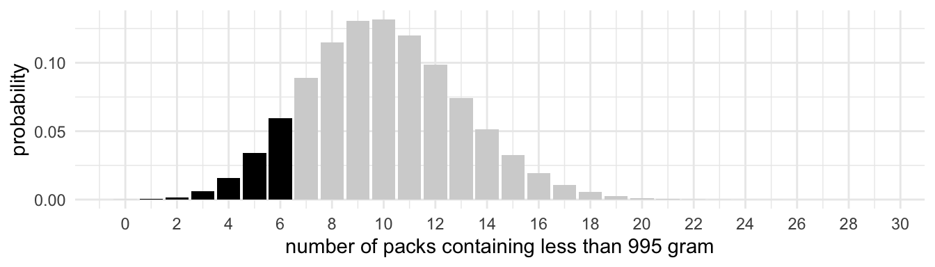

The black area corresponds with the probability of 6 or less successes in 100 trials under the assumption that the probability of a success equals 0.10.

The prob-value in this case equals .117. In other words, at a .05 significance level, the data do not support the hypothesis that less than 10% op the packs contain less than 995 grams. So the data do not give support to the hypothesis that the new machine is better. This does not mean that the new machine is not better than the old one; it does say that the collected data do not give ‘statistical evidence’ that the new machine is better.

Question: for which numbers of packages in the sample that contain less than 995 gram, would the H₀-hypothesis be rejected?

Note that if the data is expanded the conclusion can change. E.g. if n = 200 and k = 12 the result would be significant (prob-value = .032).

Writing it up

Scientific reports use a standard for many aspects of the report, among which referencing, format for tables and figures and formatting text. A commonly used style is APA style, see this webpage.
APA style also applies to reporting results of hypothesis testing.
In the last example the result can be reported as follows.
Based on a one-sided binomial test the observed values (N = 100, K = 6) do not give significant support to the assumption that less than 10 percent of the packages filled by this machine, contain less than 1000 grams, p = .117.

Proportion test: comparing two groups

In a statistical analysis it is quite common to compare different groups. For instance the differences between incomes in the profit and the not-for-profit sector, the air quality in different cities, and so on.
Comparing proportions in two different groups can sometimes be used to operationalize a research question about differences between two groups.

Example: influence website background on users
In an experiment data is collected about the influence of background colors on the attractiveness of a website. Attractiveness has been operationalized by the proportion of visitors that click on a button for more information.
The same information was presented on two different backgrounds (I and II). From former research it was expected that website I is more attractive than website II.
Data collected: of the 250 visitors to the website with background I, 40 have pressed a click button to get more information; of the 225 visitors to the website with background II, 25 pressed the button.
The question is whether this data support the hypothesis that background I is more attractive.
In a statistical sence, the hypothesis to be tested is:
H_A: p_I > p_II; where p₁ is the proportion visitors of website I that clicks on the button and p_II the proportion of website II that clicks on this button.
This is an example of a two sample proportion test.
To find out if the data support the H_A-hypothesis, the probability is calculated that assuming H₀ is true, a difference between the two proportions will be found as has been found in the collected data.² THe p-value can be calculated with R’s prop.test() function:

p-value = prop.test(x=c(40,25), n=c(250,225), alternative = “greater”).

The conclusion would be: a one-sided two-independent-samples proportion test did not support the assumptiom that visitors of website I significantly more often click the button (N = 250, K = 40, proportion = .160) than visitors of website II do (N = 225, K = 25, proportion = .111), p = .079.

The example is inspired by the interview in this podcast ↩︎
The mathematical background behind this calculation is based on the distribution of all possible differences between p₁ and p₂ in two samples, under the assumption that in real the two proportions are the same. Under the condition that the sample sizes are not too small, this distribution is a normal distribution.↩︎